Photo Credit

Original Medium Blog Link

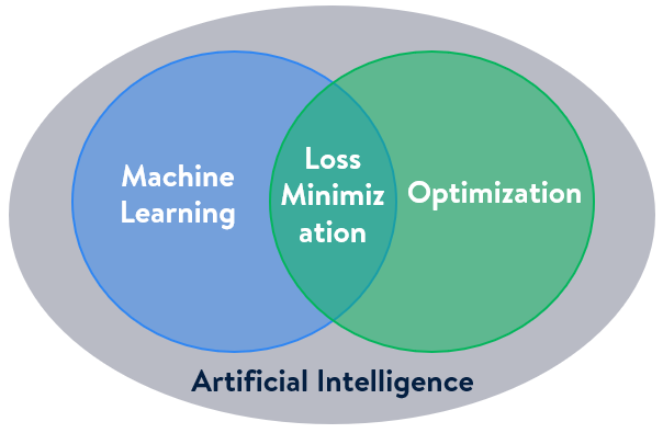
Optimization refers to finding the values of inputs in such a way that we get the best output values. The set of all possible solutions or values which the inputs can take makes up the search space. The aim of optimization is to find a point or set of points in the search space that gives the optimal solution. Amid the buzz of machine learning, the importance of optimization is overlooked oftentimes. However, optimization is a key ingredient in the recipe of machine learning algorithms. It begins with defining some kind of loss/cost function and ends with minimizing that function. For example, in the least-square regression method, the goal is to obtain the best line of fit by minimizing the sum of the square of errors.

Over the years, various types of methods have been developed to solve a wide variety of optimization problems. Genetic Algorithm (GA) is one such method that has the ability to deliver a “good-enough” solution “fast-enough” in large-scale problems, where traditional algorithms might fail to deliver a solution. It is a search-based algorithm based on the principles of genetics and natural selection which is particularly useful for solving subset selection, scheduling types of problems. In this article, an introductory overview of the genetic algorithm process along with a couple of examples from subset selection problem types is explained.

By the end of this article, you’ll know about:

• overview of how an optimization problem is formulated,
• challenges of solving optimization problems and how GA can help,
• structure of the GA in single-objective optimization problems,
• implementation of GA using a python library with an example from real-estate use cases.

1. Introduction to Optimization Problem

An optimization problem with only a single objective has the following mathematical form:

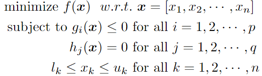
Here, the vector x of length n is the decision variable of the optimization problem, the function f is the objective function, the functions g_1, g_2,…, g_p are the inequality constraint functions, and h_1, h_2,…, h_q are the equality constraint functions. Each of the decision variables can also be individually subject to other constraints such as lower (l_k) and/or upper (u_k) bounds as well as to constraints of being discrete or continuous values, etc. It is noteworthy to mention that the above minimization problem can also be converted to a maximization problem just by reversing the sign of the objective function f.

Let’s take a well-known combinatorial optimization problem called the ‘0–1 Knapsack Problem’ for example. This problem appears in a wide variety of real-world decision-making processes, such as resource allocation, selection of investments and portfolios, etc.

[Image Credit: Wikipedia](https://en.wikipedia.org/wiki/Knapsack_problem)

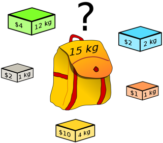
Let’s consider you are going on a hiking trip and you want to carry some useful items in your knapsack (bag) for the trip. There are five items to choose from and you know the values (v) and weights (w) of all the items. Also, you cannot take all of them since the knapsack has a maximum weight capacity. So, now you have to decide which items to pick and which ones to leave out. The objective is to maximize the total value of the selected items while staying under the weight limit. Mathematically, the above-mentioned knapsack item selection problem will have the following form:

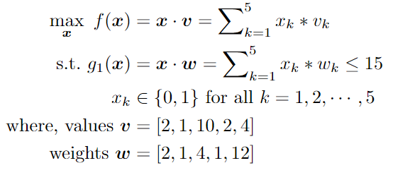
Here, the decision variable x_k can either be 1 or 0, which indicates whether the k-th item is picked or not, respectively. Optimization problems of this type of mathematic form are known as ‘binary programming’, which is a special case of ‘integer programming’. Next, we are going to dive into the challenges that may arise in solving optimization problems.

2. Challenges in Solving Optimization Problem

First, let’s try to solve the combinatorial knapsack problem using the most naive approach possible known as “brute-force”, where we exhaustively try all the possible combinations for decision variable x from search space, compute the corresponding objective function values and feasibility based on the weight constraint, and determine the best solution accordingly. In this case, for each of the 5 items, we have 2 possible decisions/inputs; 1 or 0. From combinatorics theory, we know the total number of possible combinations is 2^5=32. After iteratively going through all the combinations, we find the optimal solution is x = [1, 1, 1, 1, 0], which returns the total value of $15 with the total weight being 8 kg.

However, as you keep increasing the size of the problem, i.e., the number of items (n), the computational complexity is going to increase exponentially. For example, for n=40 items, we’ll have a total of 1 trillion combinations! Even the best supercomputer in the world will take years to evaluate all of them. So, obviously, the “brute-force” approach is not feasible in most of the real-world optimization problems. Hence, mathematicians have been developing different types of techniques to solve complex optimization problems for many years. Moreover, there is no “one-size-fits-all” method that can guarantee you the best solution for all the different types of problems. The choice of algorithm depends on the type of the problem as various algorithms are developed with specific structures keeping in mind specific problems. Readers are encouraged to read the article in this link to get an overview of different classes of optimization algorithms and to understand which one is appropriate to use in which scenarios.

Optimization algorithms can be broadly categorized based on the fact that whether the objective is a differentiable function or not. A differentiable function is a function where the gradient (derivative or slope) can be calculated for any given point in the input space. This divides algorithms into those that can make use of the calculated gradient information and those that do not. The so-called “classical” optimization algorithms such as the bisection method, newton’s method, gradient descent, etc. use the derivative information in order to obtain an optimal solution. Although gradient-based methods tend to converge significantly faster on smooth functions than gradient-free methods, gradient-based algorithms suffer from the following problems:

• difficult to apply to non-differentiable or discontinuous objective functions.
• the inherent tendency of getting stuck at local optima when the objective function is non-convex (i.e. multiple valleys and peaks)

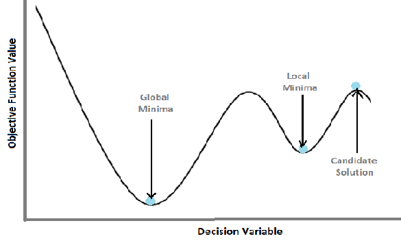
Hence, considering the complexity of real-world problem scenarios, gradient-free algorithms prove to be the better choice oftentimes. The genetic algorithm comes from a class of algorithms known as “evolutionary or population algorithms” that do not require the gradient of the objective function. This method can be used to solve a variety of optimization problems that are not well suited for standard optimization algorithms, including problems in which the objective function is discontinuous, non-differentiable, stochastic, or highly nonlinear. Next, we’ll walk through different steps of a conventional genetic algorithm using the knapsack example.

3. Structure of a Genetic Algorithm with Single Objective

First, it is essential to be familiar with some basic terminology associated with genetic algorithms.

GA terminology

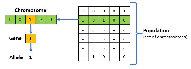
• Chromosome − A chromosome is one particular solution to the given problem. The size of the chromosome is determined by the size of the decision variable x.
• Gene − A gene is one element position of a chromosome, i.e. a single element of the decision variable.
• Allele − It is the value a gene takes for a particular chromosome. For e.g., in the knapsack problem, the allele could be either 1 or 0.
• Population − It is a subset of all the possible solutions to the given problem. The population for a GA is analogous to the population for human beings in the sense that a candidate solution can be represented as an individual. One important parameter for the GA is the population_size which is influenced by the complexity of the problem. The same size of the population is maintained throughout all the generations. The more parameters we need to optimize, the larger the population is preferred.

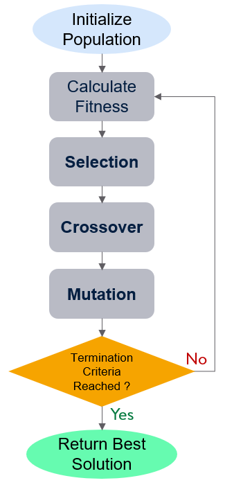
Flowchart of the genetic algorithm process

Population Initialization: There are two initialization methods-

1. Random- populate with completely random solutions.
2. Heuristic- populate using a known heuristic for the problem.

It is advisable not to initialize the entire population with a heuristic, as it can result in the population having similar solutions and very little diversity. It has been experimentally observed that the random solutions are the ones to drive the population to optimality. Therefore, with heuristic initialization, we just seed the population with a couple of good solutions, filling up the rest with random solutions.

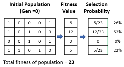
Fitness Function: The fitness function evaluates how “fit” our how “good” a candidate solution is with respect to the problem. Calculation of fitness value is done repeatedly in a GA and therefore it should be sufficiently fast.

In most cases, the fitness function and the objective function are the same as the objective is to either maximize or minimize the given objective function. However, for more complex problems with multiple objectives and constraints, different techniques might be required to design the fitness function, such as weighted summation of multiple objective functions, treating violation of constraints as a penalty, etc.

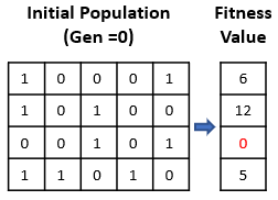
For our knapsack problem, let’s set the population_size=4 and initialize the population (generation=0 ) as depicted in the above figure. It can be observed that 3rd candidate solution is given a fitness score of 0. This is because, according to the 3rd solution, if item #3 and item#5 are picked, the total weight will be 16 which violates the weight capacity constraint, thus making it a bad/infeasible solution.

Parent Selection: In this step, parent solutions from the current generation are selected which mate and recombine to create off-springs for the next generation. Parent selection is very crucial to the convergence rate of the GA as good parents drive individuals to better and fitter solutions. However, maintaining good diversity in the population is also extremely crucial for the success of a GA, so that one extremely fit solution is prevent from taking over the entire population in a few generations.

Details of different selection techniques can be found here. To give an example, we apply the “Roulette Wheel Selection” technique. In this technique, every individual can become a parent with a probability that is proportional to its fitness. The probability is the ratio of an individual’s fitness to the total fitness of the population. Therefore, fitter individuals have a higher chance of mating and propagating their genes to the next generation.

Crossover: This is analogous to reproduction and biological crossover. Here, usually, two parents (chromosomes) are selected and one or more off-springs are produced by crossing over the genes of the parents. As a result, the off-springs can be potentially better than their parents by inheriting good genes from both parents and similarly be worse by getting bad genes. This operation is controlled by a parameter called crossover_probabilitywhich is usually set to a very high value of close to 1. The parent selection and crossover operations are repeated multiple times until the number of the solutions in the next generation reaches the population_size .

Different crossover methods are described here. For example, in the “one-point crossover” method, a random crossover point is selected and the tails of its two parents are swapped to get two new off-springs. In the following figure, the crossover operations resulted in getting a better solution with a fitness value of 14 as well as a worse solution with a fitness value of only 3.

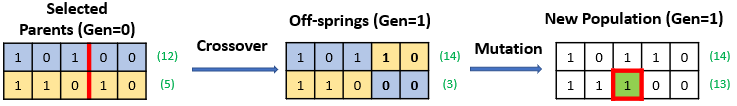
Mutation: It can be defined as a small random tweak in the chromosome, to get a new solution. It is used to maintain and introduce diversity in the population and is usually applied with a low mutation_probability (e.g. <0.1). Various techniques for mutation can be found here. In the above example, we have applied the “bit flip mutation”, where we select one or more random bits and flip them. This is used for binary-encoded GAs. Here we can observe that only one bit in only one chromosome was flipped which resulted in a significant improvement in the fitness value from 3 to 13.

Termination: The algorithm is terminated when one of the following criteria is met:

• if a known optimal or acceptable solution level is attained
• if a maximum number of generations have been performed
• if a given number of generations without fitness improvement occur

Like other parameters of a GA, the termination condition is also highly problem-specific. After the iterative process is terminated, we return the best solution from the last generation of the population.

4. Store Site Selection in Python using GA

For demonstrating how to implement a genetic algorithm using python packages, we consider a new problem from the real estate use cases. Let’s assume, you are a strategic decision leader in a retail company and your company is looking forward to expanding its business by opening new stores. You select a suitable region and find some potential sites/locations for building new stores where NUM_LOC denotes the total number of potential locations. Similar to the knapsack problem, here you have to decide which are the best locations to build new stores with different financial constraints (to be discussed later) taken into consideration just like the weight capacity constraint. However, not only do you have to decide the location, but also what format/type of store to be built at a particular location, where NUM_FMT denotes the number of possible formats. So the difference with the knapsack problem is that our decision is now two-dimensional: which location and what format. The decision variable x can be defined in either of two ways:

1. Length of variable is determined only by the number of locations such that x = [x_1, x_2, …, x_NUM_LOC], where x_k denotes the decision for k-th location. The possible values of x_k is dependent on the number of formats, such that x_k could take any integer value between 0 and NUM_FMT. For example, x_k=0 means that k-th location is not selected, x_k=1 means k-th location is selected for building store for format #1, and so on. This approach will turn the problem to be “integer programming”.
2. If we want to frame the problem as “0–1 integer programming” just like the knapsack example, then we’ll have to encode our input (candidate solution) as shown below. As a result, the length of x = NUM_LOC*NUM_FMT . For the sake of this example, let’s adopt this approach.

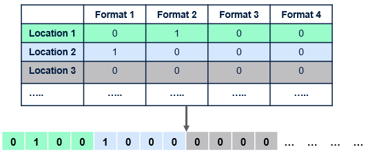
Encoding of a sample solution from two-dimensional decision to one-dimension

The problem takes four (4) financial estimations into consideration as inputs- sales, costs, net present value, and cannibalization impact of building a particular store format in a given location. Keeping consistent with the structure of our decision variable, we also need to encode our financial variables as a one-dimensional array.

import numpy as np
NUM_LOC = 3 # Numebr of possible store locations  
NUM_FMT = 3 # Number of store formats/types  
## Matrices for Financial Estimates (in Millions)  
# Sales  
S_mat = np.array([[75, 50, 25], [70, 40, 20], [65, 35, 15]])  
# Costs   
C_mat = np.array([[35, 20, 10], [35, 20, 10], [30, 18, 8]])       
# NPV  
N_mat = np.array([[10, 6, 4], [10, 5, 3], [9, 5, 3]])  
# Impact  
I_mat = np.array([[3, 2, 1], [3, 2, 1], [3, 2, 1]])  
# Vector Representations  
sales, cost, npv, impact = S_mat.flatten(), C_mat.flatten(), N_mat.flatten(), I_mat.flatten()

In addition, the following business constraints are set.

• Total costs of the selected stores ≤ CAPEX_LIMIT
• Total sales of the selected stores ≥ MIN_MARKET_SALES
• Only 1 store format is allowed in each location (if the location is picked)

# Business Constraint (in Millions)  
CAPEX_LIMIT = 55    # Capital Expenditure Limit                            
MIN_MKT_SALES = 105  # Minimum Sales from market

Now that all the variables have been set up we can define our problem as a class object. In this demonstration, we’ll be using a package called “pymoo” to solve this problem via GA. First, we initialize the ‘problem’ class with different parameters such as the size of the decision variable (n_var), number of objective functions (n_obj), number of constraints (n_constr), upper and lower bounds of decision variable (xu,xl ), and type of variable.

#%% Importing Libraries  
from pymoo.factory import get_algorithm, get_crossover, get_mutation, get_sampling  
from pymoo.optimize import minimize  
from pymoo.core.problem import Problem#%% Problem Definiton  
class MyProblem(Problem):  
    # Definition of a store site selection problem  
    def __init__(self):  
        super().__init__(n_var = NUM_LOC*NUM_FMT,  
                         n_obj = 1,  
                         n_constr = NUM_LOC+2,  
                         xl = 0,  
                         xu = 1,  
                         type_var = int)

Next, we define the objective function and the constraints. In this problem scenario, we aim to maximize the value of (NPV of selected stores — Imapct of selected stores ) and set it as our fitness function.

con_mat = np.zeros((NUM_FMT*NUM_LOC, NUM_LOC), dtype=int)  
for i in range(NUM_LOC):      
	  con_mat[i*NUM_FMT:(i+1)*NUM_FMT,i] = 1def _evaluate(self, X, out, *args, **kwargs):  
      # Objective and Constraint functions  
      out["F"] = -np.sum(X*(npv-impact), axis=1)  # Objetive Value  
      g1 = np.sum(X*cost, axis=1)- CAPEX_LIMIT  # CAPEX constraint  
      g2 = -(np.sum(X*sales, axis=1) - MIN_MKT_SALES)#SALES constraint  
      g3 = (X@con_mat) -1 # max 1 store format per location  
      out["G"] = np.column_stack([g1, g2, g3])

Finally, we call the GA to solve this custom-defined problem. We set pop_size=20, crossover_probability=1, and number of total genreation=30 for terminating the process.

#%% Solution  
method = get_algorithm("ga",                         
             pop_size=20,  
             sampling=get_sampling("int_random"),  
             crossover=get_crossover("int_sbx", prob=1.0, eta=3.0),  
             mutation=get_mutation("int_pm", eta=3.0),  
             eliminate_duplicates=True,)res = minimize(MyProblem(),  
               method,  
               termination=('n_gen', 30),  
               seed=1,  
               save_history=True)   
print("Best solution found: %s" % res.X)  
print("Function value: %s" % res.F)  
print("Constraint violation: %s" % res.CV)  
=================================================================# Result:  
Best solution found: [0 0 1 0 0 1 1 0 0]  
Function value: [-11.]  
Constraint violation: [0.]

The entire code is available here. After we decode the result, it is evident that the best solution for this toy example is to build a Format-3 store at Location-1, a Format-3 store at Location-2, and a Format-1 store at Location-3.

5. Conclusion

GA is an efficient tool to find optimal or near-optimal solutions to difficult problems in a short amount of time. While the algorithm has proven to be more suitable for optimization problems like scheduling and subset selection, the efficiency of the method mostly depends on how well the problem is defined through chromosomes and how well the solutions are evolving across generations. In the next part, we’ll learn about different variations of the genetic algorithm and how the structure differs while solving multi-objective optimization problems.

6. References

• Knapsack problem - Wikipedia
• Integer programming - Wikipedia
• How to Choose an Optimization Algorithm - Machine Learning Mastery
• Genetic Algorithms - Tutorialspoint
• pymoo: Multi-objective Optimization in Python